
The Corner Bean is a bistro located on a major highway’s gas station. Most of its customers are new, one time customers like drivers and passengers on long trips, who may stop by for quick snacks, full meals, or just coffee — choices that vary with their hunger, time constraints, and even road conditions. These interaction of variables would create uncertainty in the amount any customer could spend.
However, for the owner of The Corner Bean, this creates a dilemma:
- How can he estimate how much a customer could spend in a single interaction?
- How can he estimate how much revenue he could earn in a week?
Answering these questions seem to be quite an uphill task given the amount the next customer could spend feels almost random.
To attempt to answer these questions, we might perhaps take inspiration from other phenomena that exhibit random behavior; rolling a die.
If we roll a fair die the result of any single roll is entirely random, you could get a 6, 4, or a 1. In probability theory, we model this as a probability distribution, a uniform distribution where each possible outcome — 1, 2, 3, 4, 5, or 6 — has an equal probability, 1/6, of happening.
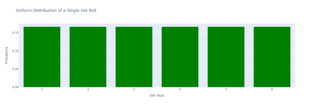
So, if we wanted to predict that the outcome of a roll will be a 6, there’s little certainty that we’ll see it, the prediction will be a gamble at best.
Now, let’s change things up. Suppose we increase the number of rolls to 2, and instead of predicting the outcome of a single die, we’re interested in predicting the sum of the two rolls.
The possible outcomes now range from 2 (rolling two 1s) to 12 (rolling two 6s). However, the probabilities for these sums are no longer equal. The probability distribution shifts dramatically.
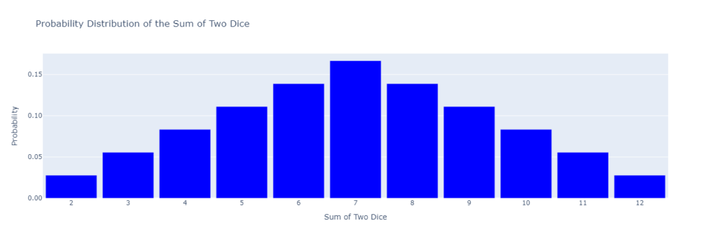
Some sums, like 7, are much more likely than others, like 2 or 12.
Why?
Think about it intuitively. To roll a sum of 12, both rolls of the die must show a 6 — there’s only one combination that achieves this: {6, 6}. The same applies to rolling a 2, which requires {1, 1}.
However, there are multiple combinations that can produce the sum 7: {1, 6}, {2, 5}, {3, 4} — a total of 3 possibilities.
This makes rolling a 7 far more likely than rolling a 2 or 12. The same logic applies to other mid-range sums like 6 or 8, where more combinations exist to produce the result.
So, If we were to make a bet, like in the beginning, our odds are better choosing a 7 than a 12.
Increasing the rolls to 50, the probabilities of the sums get further from being evenly distributed, growing exponentially for mid-range values and while diminishing for extreme values.
For instance, the probability of rolling the lowest possible sum, 50, requires all 50 dice rolls to show 1 — a single combination out of millions. Similarly, achieving the maximum sum of 300 requires all 50 dice rolls to show 6, which is just as rare.
But for a mid-range sum, like 175. Well, there are countless ways this could occur: some dice might roll high numbers like 5 or 6, while others roll lower values like 1 or 2. These variations create an overwhelming number of combinations that contribute to mid-range sums, making them vastly more likely.
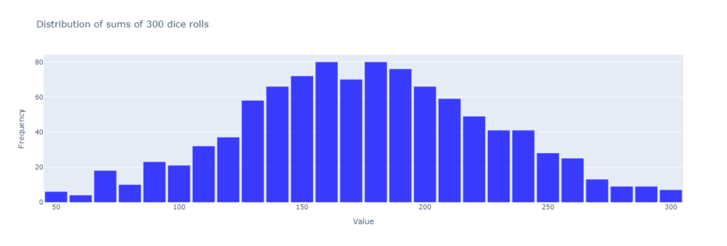
As we increase in the number of rolls — to infinity — the distribution of the sums takes on a very distinct shape, a bell curve, with more likely outcomes cluster around the middle of the range, while the extremes become increasingly unlikely.
This phenomenon, called the central limit theorem, illustrates two powerful ideas:
- The more outcomes we aggregate, random each as each might be, the less “random” the overall outcome appears.
- The central limit theorem holds regardless of the underlying distribution of data. (whether it is the uniform distribution we’ve seen above or any unknown distribution)
To apply the central limit theorem in our use case, let’s assume the underlying distribution of the observed customer spending is unknown
Suppose he treats each customer’s spending like a random draw from the underlying distribution, If he wanted to predict how much revenue the owner would earn from 100 customers in a week, the owner could:
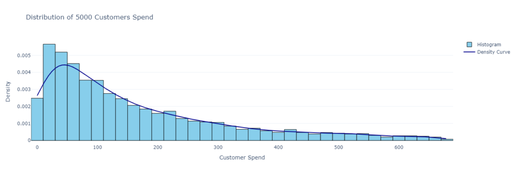
- Record spending data for a week to build a dataset of customer spending, say 5000 transactions. We could plot the distribution of the 5000 purchases as shown below:
- Therefore, each transaction is like a random draw from the distribution above.
- From the transactions, we take random samples of 100 transactions from the original data set of 5000, each transaction from a unique customer.
- Sum up the transactions amount and place it aside. (we could also instead of the sum, get the mean by dividing it by 100 then place it aside. Either of the two aggregation techniques suffices)
- We would then go back to our data and repeatedly draw samples of 100, calculating the sum/mean and placing it aside. We could repeat this as many times as we want to capture as much behavior from our original purchases distribution. We can think of each sum/mean representing a different scenarios of how different combinations of 100 customers would behave.
By using the mean, for example, the store owner captures nearly every plausible way that the average spending behavior of 100 customers could play out. The result is a distribution of sample means, known as the sampling distribution.
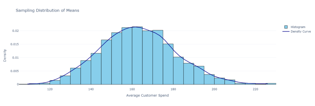
Why is this useful? Because this distribution doesn’t just reveal the most likely average revenue — it also provides insight into the range within which average customer spend is likely to fall, giving the owner a much clearer picture of financial expectations. Additionally, it displays where 100 customer spending averages out and how widely it can vary from that average.
Moreover, this distribution tends to take the shape of a normal distribution which compared to the unknown underlying distribution, is far easier to make statistical inferences from. Most customers will cluster around a typical spending range, with fewer making significantly larger or smaller purchases.
The magic of this approach lies in the nice properties that emerge from the resultant normal distribution. For example, If we use the mean , we tend to understand what on average would a customers spend.
- It enables us to gain Key Insights from answering questions like:
What is the probability that the average spending per customer is between $10 and $15 for example
2. Whereas If we use the Sum as in our dice examples, we gain Key Insights from answering questions like:
What is the probability that I would make between $1000 and $2000 if only 100 customers came to my store?
The two contributions above would help the owner of the cafe’s dilemma
The above case involves looking at monetary spend in isolation.
However, customer behavior is rarely driven by a single factor alone. A more insightful approach, would include another factor, like Duration, a variable we can define as how long a customer stays in the cafe.
Imagine that while sampling, we don’t just capture the averages of monetary spend but also how long customers stay.
This results in a sampling distribution of monetary spend and stop duration, forming a bivariate distribution — an interaction of how time spent correlates with spending.
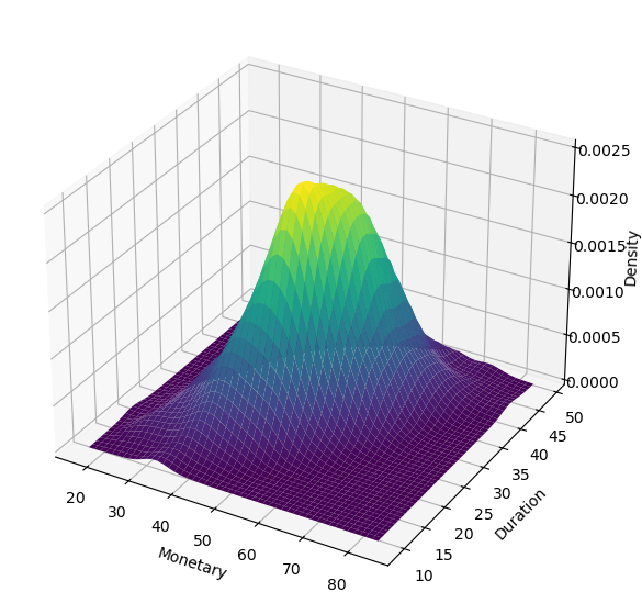
By incorporating this perspective, we unlock deeper insights that enable more nuanced predictions, such as:
- Given that a customer stops for more than 30 minutes, what is the probability that their average spend exceeds $500?
This would give a far more informative answer that could help with optimize staffing, seating, and inventory. For example, if longer stays correlate with higher spending, allocating more space for these customers may be profitable.
The assumptions we would have to make to qualify this approach would be:
- Individual customer behaviors are independent of one another. Which means, one customer’s purchase does not influence another’s behavior.
- The customer spend is relatively stationary. This, I admit is a far stronger assumption since behavior is often subject to change, which might require additional sophisticated modelling techniques like timeseries forecasting to answer the above statistical inference questions for a more accurate prediction.
Despite these assumptions, the CLT proves to be an incredible tool in predictive assessments of uncertain and seemingly random events.